Overview
cgmguru provides high-performance tools for continuous
glucose monitoring (CGM) analysis. It combines two complementary
workflows:
- consensus-style glycemic event detection for hypo- and hyperglycemia
- GRID-based detection of rapid glucose rises and postprandial maxima
This guide expands the package-level vignette into a practical
workflow. It is based on the longer
vignette("intro", package = "cgmguru") source and focuses
on how to move from a raw CGM table to subject summaries, event tables,
GRID starts, postprandial peaks, and simple visual checks.
Data Contract
Most cgmguru functions expect a data frame with these
columns:
| Column | Meaning |
|---|---|
id |
Subject identifier |
time |
POSIXct timestamp |
gl |
Glucose value in mg/dL |
Rows may contain multiple subjects. For speed and reproducibility, it
is good practice to order by id and time
before analysis, especially when chaining several functions.
data(example_data_5_subject, package = "iglu")
data(example_data_hall, package = "iglu")

cgm_data <- orderfast(example_data_5_subject)

data.frame(
  rows = nrow(cgm_data),
  subjects = length(unique(cgm_data$id)),
  first_time = min(cgm_data$time),
  last_time = max(cgm_data$time),
  min_glucose = min(cgm_data$gl, na.rm = TRUE),
  max_glucose = max(cgm_data$gl, na.rm = TRUE)
)
#>    rows subjects          first_time           last_time min_glucose
#> 1 13866        5 2015-02-24 17:31:29 2015-06-19 08:59:36          50
#>   max_glucose
#> 1         400
cat("The 'iglu' package is not available, so example-data chunks are skipped.\n")Two Preprocessing Models
The package intentionally separates event-grid analysis from GRID-family analysis.
Glycemic event functions use an iglu-compatible event grid:
These functions can infer reading_minutes per subject
from the median positive timestamp spacing. They align to a full-day
grid, interpolate gaps up to inter_gap, remove larger
gap-masked rows, and classify events by contiguous segments.
GRID-family functions operate on the rows you pass in:
They do not automatically call the event-grid interpolation pipeline. If you want GRID analysis on an interpolated series, explicitly pass the interpolated data.
Subject-Level Overview
sensor_wear() calculates how much observed CGM data are
present. By default it uses each subject’s original timestamp span.
Supplying ndays switches to a fixed retrospective window
ending at each subject’s last valid timestamp, or at a common
end_date if you provide one.
sensor_wear(cgm_data, reading_minutes = 5)
#> # A tibble: 5 × 6
#>   id        sensor_wear_percent sensor_wear ndays start_date
#>   <chr>                   <dbl>       <dbl> <dbl> <dttm>
#> 1 Subject 1                79.8        79.8    NA 2015-06-06 16:50:27
#> 2 Subject 2                58.9        58.9    NA 2015-02-24 17:31:29
#> 3 Subject 3                92.1        92.1    NA 2015-03-10 15:36:26
#> 4 Subject 4                98.7        98.7    NA 2015-03-13 12:44:09
#> 5 Subject 5                95.8        95.8    NA 2015-02-28 17:40:06
#> # ℹ 1 more variable: end_date <dttm>

sensor_wear(cgm_data, ndays = 14, reading_minutes = 5)
#> # A tibble: 5 × 6
#>   id        sensor_wear_percent sensor_wear ndays start_date
#>   <chr>                   <dbl>       <dbl> <dbl> <dttm>
#> 1 Subject 1                72.3        72.3    14 2015-06-05 08:59:36
#> 2 Subject 2                51.1        51.1    14 2015-02-27 09:38:01
#> 3 Subject 3                38.0        38.0    14 2015-03-02 10:11:05
#> 4 Subject 4                90.9        90.9    14 2015-03-12 10:01:58
#> 5 Subject 5                72.5        72.5    14 2015-02-25 08:04:28
#> # ℹ 1 more variable: end_date <dttm>
For a broader one-row-per-subject summary, use
detect_all_events().
all_events <- detect_all_events(
cgm_data,
reading_minutes = 5,
sensor_wear_ndays = 14
)
names(all_events)
#> [1] "subject_summary" "glycemic_event_summary"
head(all_events$subject_summary)
#> # A tibble: 5 × 24
#> id TIR TITR TBR70 TBR54 TAR180 TAR250 CV SD mean_glucose GMI
#> <chr> <dbl> <dbl> <dbl> <dbl> <dbl> <dbl> <dbl> <dbl> <dbl> <dbl>
#> 1 Subject 1 91.7 73.7 0.14 0 8.2 0.38 26.9 33.3 124. 6.27
#> 2 Subject 2 26.4 3.36 0 0 73.6 26.1 24.0 52.4 218. 8.54
#> 3 Subject 3 81.3 49.8 0.33 0 18.3 5.68 29.1 44.8 154. 6.99
#> 4 Subject 4 95.1 67.7 0.27 0.05 4.61 0 22.4 29.1 130. 6.41
#> 5 Subject 5 62.1 30.1 0.1 0 37.8 11.3 33.6 58.6 175. 7.49
#> # ℹ 13 more variables: uGMI <dbl>, GRI <dbl>, sensor_wear_percent <dbl>,
#> # hypo_lv1_total_episodes <int>, hypo_lv2_total_episodes <int>,
#> # hypo_extended_total_episodes <int>, hypo_lv1_excl_total_episodes <int>,
#> # hypo_rebound_total_episodes <int>, hyper_lv1_total_episodes <int>,
#> # hyper_lv2_total_episodes <int>, hyper_extended_total_episodes <int>,
#> # hyper_lv1_excl_total_episodes <int>, hyper_rebound_total_episodes <int>
head(all_events$glycemic_event_summary)
#> # A tibble: 6 × 6
#> id type level total_episodes avg_ep_per_day avg_minutes_below_54_…¹
#> <chr> <chr> <chr> <int> <dbl> <dbl>
#> 1 Subject 1 hypo lv1 1 0.09 0
#> 2 Subject 1 hypo lv2 0 0 0
#> 3 Subject 1 hypo extended 0 0 0
#> 4 Subject 1 hypo lv1_excl 1 0.09 0
#> 5 Subject 1 hypo rebound 0 0 0
#> 6 Subject 1 hyper lv1 16 1.44 0
#> # ℹ abbreviated name: ¹avg_minutes_below_54_per_episodeThe subject_summary table includes CGM summary metrics
such as time in range, time below range, time above range, mean glucose,
variability, GMI/uGMI, GRI, and sensor_wear_percent. By
default, these summary glucose metrics are calculated from the original
raw glucose values. Set
summary_metrics_source = "preprocessed" to calculate them
from the internal event grid after interpolation and gap masking.
all_events_preprocessed <- detect_all_events(
  cgm_data,
  reading_minutes = 5,
  summary_metrics_source = "preprocessed"
)

head(all_events_preprocessed$subject_summary)
#> # A tibble: 5 × 24
#>   id          TIR  TITR TBR70 TBR54 TAR180 TAR250    CV    SD mean_glucose   GMI
#>   <chr>     <dbl> <dbl> <dbl> <dbl>  <dbl>  <dbl> <dbl> <dbl>        <dbl> <dbl>
#> 1 Subject 1  91.8 74.0   0.16  0      8.08   0.37  26.7  33.0         123.  6.26
#> 2 Subject 2  25.8  3.28  0     0     74.2   26.5   24.1  52.6         219.  8.54
#> 3 Subject 3  81.3 49.8   0.32  0     18.4    5.44  29.0  44.5         154.  6.98
#> 4 Subject 4  94.9 67.4   0.33  0.03   4.75   0     22.4  29.0         130.  6.41
#> 5 Subject 5  62.0 29.6   0.1   0     37.9   11.5   33.4  58.4         175.  7.49
#> # ℹ 13 more variables: uGMI <dbl>, GRI <dbl>, sensor_wear_percent <dbl>,
#> #   hypo_lv1_total_episodes <int>, hypo_lv2_total_episodes <int>,
#> #   hypo_extended_total_episodes <int>, hypo_lv1_excl_total_episodes <int>,
#> #   hypo_rebound_total_episodes <int>, hyper_lv1_total_episodes <int>,
#> #   hyper_lv2_total_episodes <int>, hyper_extended_total_episodes <int>,
#> #   hyper_lv1_excl_total_episodes <int>, hyper_rebound_total_episodes <int>
Inspecting the Event Grid
When you need to audit event boundaries, use
return_interpolated = TRUE. The returned
interpolated_data is the grid used internally for event
classification.
all_events_with_grid <- detect_all_events(
  cgm_data,
  reading_minutes = 5,
  return_interpolated = TRUE
)

names(all_events_with_grid)
#> [1] "subject_summary"        "glycemic_event_summary" "interpolated_data"
head(all_events_with_grid$interpolated_data)
#> # A tibble: 6 × 3
#>   id        time                   gl
#>   <chr>     <dttm>              <dbl>
#> 1 Subject 1 2015-06-06 16:55:00  148.
#> 2 Subject 1 2015-06-06 17:00:00  143.
#> 3 Subject 1 2015-06-06 17:05:00  137.
#> 4 Subject 1 2015-06-06 17:10:00  129.
#> 5 Subject 1 2015-06-06 17:15:00  122.
#> 6 Subject 1 2015-06-06 17:20:00  121.
The standalone helper interpolate_cgm() is useful when
you want to inspect preprocessing before running event detectors.
event_grid <- interpolate_cgm(cgm_data, reading_minutes = 5)
head(event_grid)
#> # A tibble: 6 × 3
#>   id        time                   gl
#>   <chr>     <dttm>              <dbl>
#> 1 Subject 1 2015-06-06 16:55:00  148.
#> 2 Subject 1 2015-06-06 17:00:00  143.
#> 3 Subject 1 2015-06-06 17:05:00  137.
#> 4 Subject 1 2015-06-06 17:10:00  129.
#> 5 Subject 1 2015-06-06 17:15:00  122.
#> 6 Subject 1 2015-06-06 17:20:00  121.
Hypoglycemia and Hyperglycemia Events
Use the standalone event functions when you need detailed event
boundaries for one event type. Presets are available through
type = "lv1", "lv2", "extended",
and "lv1_excl".
hyper_lv1 <- detect_hyperglycemic_events(
  cgm_data,
  type = "lv1",
  reading_minutes = 5,
  return_interpolated = FALSE
)

hypo_lv1 <- detect_hypoglycemic_events(
  cgm_data,
  type = "lv1",
  reading_minutes = 5,
  return_interpolated = FALSE
)

hyper_lv1$events_total
#> # A tibble: 5 × 3
#>   id        total_episodes avg_ep_per_day
#>   <chr>              <int>          <dbl>
#> 1 Subject 1             16           1.44
#> 2 Subject 2             21           2.13
#> 3 Subject 3              9           1.64
#> 4 Subject 4             13           1.02
#> 5 Subject 5             38           3.72
hypo_lv1$events_total
#> # A tibble: 5 × 3
#>   id        total_episodes avg_ep_per_day
#>   <chr>              <int>          <dbl>
#> 1 Subject 1              1           0.09
#> 2 Subject 2              0           0
#> 3 Subject 3              1           0.18
#> 4 Subject 4              2           0.16
#> 5 Subject 5              1           0.1
head(hyper_lv1$events_detailed)
#> # A tibble: 6 × 7
#>   id        start_time          start_glucose end_time            end_glucose
#>   <chr>     <dttm>                      <dbl> <dttm>                    <dbl>
#> 1 Subject 1 2015-06-11 15:45:00          193. 2015-06-11 16:50:00        187.
#> 2 Subject 1 2015-06-11 17:25:00          195. 2015-06-11 19:00:00        183.
#> 3 Subject 1 2015-06-11 19:20:00          181. 2015-06-11 19:45:00        187.
#> 4 Subject 1 2015-06-11 22:35:00          187. 2015-06-11 23:45:00        185.
#> 5 Subject 1 2015-06-12 07:50:00          181. 2015-06-12 09:15:00        181.
#> 6 Subject 1 2015-06-13 16:55:00          180. 2015-06-13 18:25:00        186.
#> # ℹ 2 more variables: start_index <int>, end_index <int>
detect_all_events() is usually the most convenient
interface for reporting, because it aggregates hypo- and hyperglycemia
definitions in one call.
nonzero_events <- all_events$glycemic_event_summary[
all_events$glycemic_event_summary$total_episodes > 0,
]
head(nonzero_events)
#> # A tibble: 6 × 6
#> id type level total_episodes avg_ep_per_day avg_minutes_below_54_…¹
#> <chr> <chr> <chr> <int> <dbl> <dbl>
#> 1 Subject 1 hypo lv1 1 0.09 0
#> 2 Subject 1 hypo lv1_excl 1 0.09 0
#> 3 Subject 1 hyper lv1 16 1.44 0
#> 4 Subject 1 hyper lv2 2 0.18 0
#> 5 Subject 1 hyper lv1_excl 14 1.26 0
#> 6 Subject 2 hyper lv1 21 2.13 0
#> # ℹ abbreviated name: ¹avg_minutes_below_54_per_episodeGRID Analysis
The GRID (Glucose Rate Increase Detector) workflow detects rapid glucose rises, often used as candidate meal or postprandial start points.
grid_result <- grid(cgm_data, gap = 15, threshold = 130)

grid_result$episode_counts
#> # A tibble: 5 × 2
#>   id        episode_counts
#>   <chr>              <int>
#> 1 Subject 1             10
#> 2 Subject 2             22
#> 3 Subject 3              7
#> 4 Subject 4             18
#> 5 Subject 5             42
head(grid_result$episode_start)
#> # A tibble: 6 × 4
#>   id        time                   gl index
#>   <chr>     <dttm>              <dbl> <int>
#> 1 Subject 1 2015-06-11 15:30:07   143   966
#> 2 Subject 1 2015-06-11 17:10:07   157   985
#> 3 Subject 1 2015-06-11 22:00:06   135  1038
#> 4 Subject 1 2015-06-11 22:25:06   162  1043
#> 5 Subject 1 2015-06-12 07:40:04   160  1154
#> 6 Subject 1 2015-06-13 16:34:59   132  1415
head(grid_result$grid_vector)
#> # A tibble: 6 × 1
#>    grid
#>   <int>
#> 1     0
#> 2     0
#> 3     0
#> 4     0
#> 5     0
#> 6     0
Lowering the threshold or gap generally
makes detection more sensitive.
Postprandial Maxima
maxima_grid() combines GRID starts with local maxima to
identify likely postprandial peaks within a time window.
maxima_result <- maxima_grid(
  cgm_data,
  threshold = 130,
  gap = 60,
  hours = 2
)

maxima_result$episode_counts
#> # A tibble: 5 × 2
#>   id        episode_counts
#>   <chr>              <int>
#> 1 Subject 1              8
#> 2 Subject 2             18
#> 3 Subject 3              7
#> 4 Subject 4             16
#> 5 Subject 5             39
head(maxima_result$results)
#> # A tibble: 6 × 8
#>   id    grid_time grid_gl maxima_time maxima_glucose time_to_peak_min grid_index
#>   <chr> <dttm>      <dbl> <dttm>               <dbl>            <dbl>      <int>
#> 1 Subj… 2015-06-…     143 2015-06-11…            276               40        967
#> 2 Subj… 2015-06-…     135 2015-06-11…            209               50       1039
#> 3 Subj… 2015-06-…     160 2015-06-12…            210               40       1155
#> 4 Subj… 2015-06-…     132 2015-06-13…            202               60       1416
#> 5 Subj… 2015-06-…     176 2015-06-14…            227               45       1677
#> 6 Subj… 2015-06-…     166 2015-06-16…            208               65       2223
#> # ℹ 1 more variable: maxima_index <int>
For a more explicit step-by-step version of the workflow, chain the lower-level helpers.
grid_starts <- start_finder(grid_result$grid_vector)

mod_grid_result <- mod_grid(
  cgm_data,
  grid_starts,
  hours = 2,
  gap = 60
)

mod_grid_starts <- start_finder(mod_grid_result$mod_grid_vector)

max_after_result <- find_max_after_hours(
  cgm_data,
  mod_grid_starts,
  hours = 2
)

local_maxima <- find_local_maxima(cgm_data)

new_maxima <- find_new_maxima(
  cgm_data,
  max_after_result$max_index,
  local_maxima$local_maxima_vector
)

mapped_maxima <- transform_df(grid_result$episode_start, new_maxima)
between_maxima <- detect_between_maxima(cgm_data, mapped_maxima)

head(mapped_maxima)
#> # A tibble: 6 × 5
#>   id        grid_time           grid_gl maxima_time         maxima_gl
#>   <chr>     <dttm>                <dbl> <dttm>                  <dbl>
#> 1 Subject 1 2015-06-11 20:30:07     143 2015-06-11 21:10:07       276
#> 2 Subject 1 2015-06-12 03:00:06     135 2015-06-12 03:50:06       209
#> 3 Subject 1 2015-06-12 03:25:06     162 2015-06-12 03:50:06       209
#> 4 Subject 1 2015-06-12 12:40:04     160 2015-06-12 13:20:04       210
#> 5 Subject 1 2015-06-13 21:34:59     132 2015-06-13 22:34:59       202
#> 6 Subject 1 2015-06-14 22:39:55     176 2015-06-14 23:24:55       227
head(between_maxima$results)
#> # A tibble: 6 × 6
#>   id        grid_time           grid_gl maxima_time  maxima_glucose time_to_peak
#>   <chr>     <dttm>                <dbl> <dttm>                <dbl>        <dbl>
#> 1 Subject 1 2015-06-11 15:30:07     143 2015-06-11 …            276         2400
#> 2 Subject 1 2015-06-11 22:00:06     135 2015-06-11 …            158         1200
#> 3 Subject 1 2015-06-11 22:25:06     162 2015-06-11 …            209         1500
#> 4 Subject 1 2015-06-12 07:40:04     160 2015-06-12 …            210         2400
#> 5 Subject 1 2015-06-13 16:34:59     132 2015-06-13 …            202         3600
#> 6 Subject 1 2015-06-14 17:39:55     176 2015-06-14 …            227         2700
Excursion Analysis
excursion() identifies glucose excursions, defined as
rises greater than 70 mg/dL within 2 hours, excluding starts preceded by
hypoglycemia.
excursion_result <- excursion(cgm_data, gap = 15)

excursion_result$episode_counts
#> # A tibble: 5 × 2
#>   id        episode_counts
#>   <chr>              <int>
#> 1 Subject 1              9
#> 2 Subject 2             14
#> 3 Subject 3             11
#> 4 Subject 4             17
#> 5 Subject 5             34
head(excursion_result$episode_start)
#> # A tibble: 6 × 8
#>   id        time            gl maxima_time maxima_glucose time_to_peak_min index
#>   <chr>     <dttm>       <dbl> <dttm>               <dbl>            <dbl> <int>
#> 1 Subject 1 2015-06-11 …    87 2015-06-11…            170              120   949
#> 2 Subject 1 2015-06-11 …   187 2015-06-11…            267               75   982
#> 3 Subject 1 2015-06-11 …   120 2015-06-11…            202              120  1027
#> 4 Subject 1 2015-06-13 …    95 2015-06-13…            172              120  1400
#> 5 Subject 1 2015-06-14 …   113 2015-06-14…            190              120  1650
#> 6 Subject 1 2015-06-15 …    85 2015-06-15…            158              120  1896
#> # ℹ 1 more variable: maxima_index <int>
Quick Visualization
Visual checks are useful after tuning thresholds. The plot below shows one subject’s glucose trace, clinical thresholds, and GRID episode starts.
subject_id <- unique(cgm_data$id)[1]
subject_data <- cgm_data[cgm_data$id == subject_id, ]
subject_grid_starts <- grid_result$episode_start[
  grid_result$episode_start$id == subject_id,
]

ggplot2::ggplot(subject_data, ggplot2::aes(x = time, y = gl)) +
  ggplot2::geom_line(linewidth = 0.3, color = "steelblue") +
  ggplot2::geom_hline(yintercept = c(54, 70), linetype = "dashed",
                      color = "darkorange") +
  ggplot2::geom_hline(yintercept = c(180, 250), linetype = "dashed",
                      color = "firebrick") +
  ggplot2::geom_point(
    data = subject_grid_starts,
    ggplot2::aes(x = time, y = gl),
    color = "black",
    size = 1.4
  ) +
  ggplot2::labs(
    title = paste("CGM Trace and GRID Starts:", subject_id),
    x = "Time",
    y = "Glucose (mg/dL)"
  ) +
  ggplot2::theme_minimal()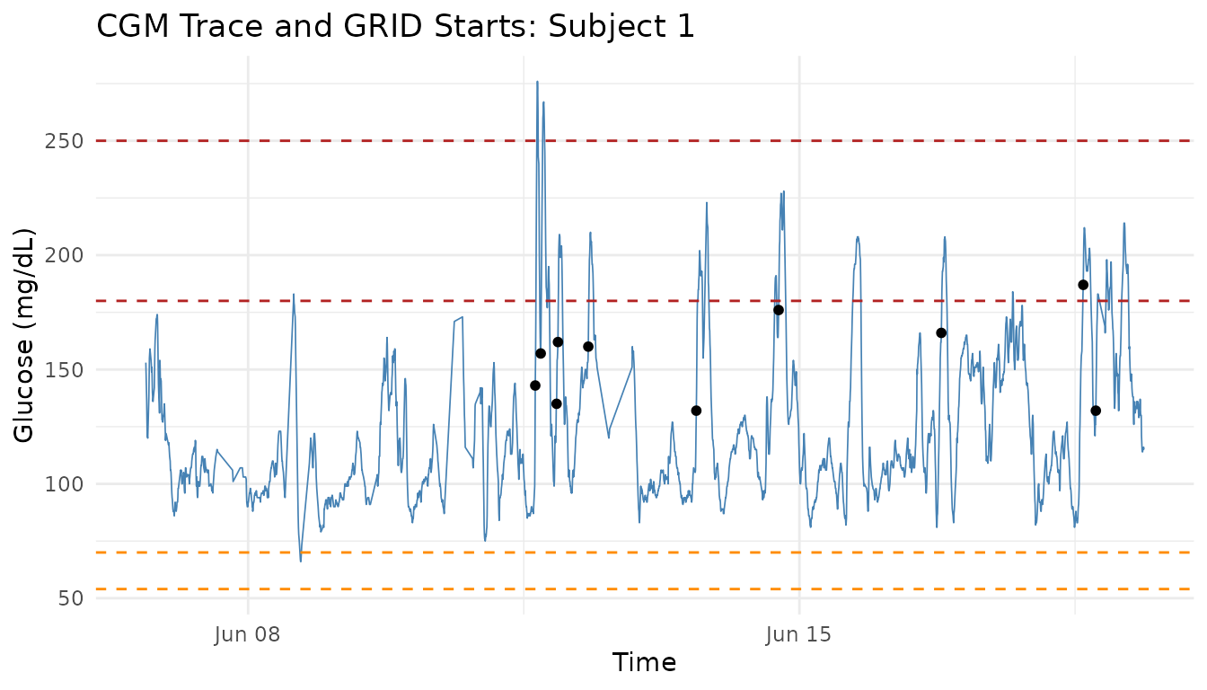
cat("The 'ggplot2' package is not available, so the plot is skipped.\n")Scaling Up
The same workflow applies to larger multi-subject datasets. The
example below uses example_data_hall from
iglu.
hall_data <- orderfast(example_data_hall)

hall_summary <- detect_all_events(hall_data, reading_minutes = 5)
hall_grid <- grid(hall_data, gap = 15, threshold = 130)

data.frame(
  subjects = length(unique(hall_data$id)),
  rows = nrow(hall_data),
  summary_rows = nrow(hall_summary$subject_summary),
  grid_rows = nrow(hall_grid$grid_vector)
)
#>   subjects  rows summary_rows grid_rows
#> 1       19 34890           19     34890
Function Map
| Task | Main function |
|---|---|
| Order CGM rows | orderfast() |
| Calculate observed data coverage | sensor_wear() |
| Build an event preprocessing grid | interpolate_cgm() |
| Report all event summaries | detect_all_events() |
| Detect one hypo/hyper event type |
detect_hypoglycemic_events(),
detect_hyperglycemic_events()
|
| Detect rapid glucose rises | grid() |
| Detect local peaks | find_local_maxima() |
| Combine GRID starts and peaks | maxima_grid() |
| Find peaks/minima around starts |
find_max_after_hours(),
find_max_before_hours(),
find_min_after_hours(),
find_min_before_hours()
|
| Refine and map postprandial peaks |
find_new_maxima(), transform_df(),
detect_between_maxima()
|
| Detect large glucose excursions | excursion() |
Next Steps
For more detailed examples, open the focused vignettes:
browseVignettes("cgmguru")
vignette("intro", package = "cgmguru")
vignette("detect_all_events", package = "cgmguru")
vignette("grid", package = "cgmguru")
vignette("maxima_grid", package = "cgmguru")
References
- Harvey RA, Dassau E, Bevier WC, et al. Design of the glucose rate increase detector: a meal detection module for the health monitoring system. Journal of Diabetes Science and Technology. 2014;8(2):307-320.
- Broll S, Urbanek J, Buchanan D, Chun E, Muschelli J, Punjabi N, Gaynanova I. Interpreting blood glucose data with R package iglu. PLoS One. 2021;16(4):e0248560.
- Chun E, Fernandes JN, Gaynanova I. An Update on the iglu Software Package for Interpreting Continuous Glucose Monitoring Data. Diabetes Technology & Therapeutics. 2024;26(12):939-950.
- Battelino T, Alexander CM, Amiel SA, et al. Continuous glucose monitoring and metrics for clinical trials: an international consensus statement. The Lancet Diabetes & Endocrinology. 2023;11(1):42-57.